why dimension reduction Dimension is the number of features. Too much dimension leads to too many effective details in order to not overfitting. So for the most of the time, data is always not enough. On the other hand, less dimension will lead to less computational time. If the information between the different sample is conserved, it means, some feature is actually deleted. So dimension reduction is actually, deleting the most unwanted features or unimportant one as a whole. Random projection Dimensionality reduction techniques generally use linear transformations in determining the intrinsic dimensionality of the manifold as well as extracting its principal directions. For this purpose there are various related techniques, including: principal component analysis, linear discriminant analysis, canonical correlation analysis, discrete cosine transform, random projection, etc. Random projection is a simple and computationally efficient way to reduce the dimensionality of data by trading a controlled amount of error for faster processing times and smaller model sizes. The dimensions and distribution of random projection matrices are controlled so as to approximately preserve the pairwise distances between any two samples of the dataset. The core idea behind random projection is given in the Johnson-Lindenstrauss lemma, which states that if points in a vector space are of sufficiently high dimension, then they may be projected into a suitable lower-dimensional space in a way which approximately preserves the distances between the points. The mathematical backaground for random projection: Johnson–Lindenstrauss lemma In mathematics, the Johnson–Lindenstrauss lemma is a result named after William B. Johnson and Joram Lindenstrauss concerning low-distortion embeddings of points from high-dimensional into low-dimensional Euclidean space. The lemma states that a small set of points in a high-dimensional space can be embedded into a space of much lower dimension in such a way that distances between the points are nearly preserved. Weakness: Though this allows some degree of visualization of the data structure, the randomness of the choice leaves much to be desired. In a random projection, it is likely that the more interesting structure within the data will be lost. Pca Principal component analysis (PCA) is a statistical procedure that uses an orthogonal transformation to convert a set of observations of possibly correlated variables into a set of values of linearly uncorrelated variables called principal components. The number of principal components is less than or equal to the number of original variables. This transformation is defined in such a way that the first principal component has the largest possible variance (that is, accounts for as much of the variability in the data as possible), and each succeeding component in turn has the highest variance possible under the constraint that it is orthogonal to the preceding components. The resulting vectors are an uncorrelated orthogonal basis set. The principal components are orthogonal because they are the eigenvectors of the covariance matrix, which is symmetric. PCA is sensitive to the relative scaling of the original variables. PCA can be thought of as fitting an n-dimensional ellipsoid to the data, where each axis of the ellipsoid represents a principal component. If some axis of the ellipse is small, then the variance along that axis is also small, and by omitting that axis and its corresponding principal component from our representation of the dataset, we lose only a commensurately small amount of information. To find the axes of the ellipse, we must first subtract the mean of each variable from the dataset to center the data around the origin. Then, we compute the covariance matrix of the data, and calculate the eigenvalues and corresponding eigenvectors of this covariance matrix. Then, we must orthogonalize the set of eigenvectors, and normalize each to become unit vectors. Once this is done, each of the mutually orthogonal, unit eigenvectors can be interpreted as an axis of the ellipsoid fitted to the data. The proportion of the variance that each eigenvector represents can be calculated by dividing the eigenvalue corresponding to that eigenvector by the sum of all eigenvalues. It is important to note that this procedure is sensitive to the scaling of the data, and that there is no consensus as to how to best scale the data to obtain optimal results. In the data science notes, you will see examples of scaling effects. So normalize using preprocessing is important!! Weakness These methods can be powerful, but often miss important non-linear structure in the data. Manifold learning - iSOMAP Due to weakness of PCA and Random Projection, a nonlinear method to learn nonlinear data structure is found.
Manifold Learning can be thought of as an attempt to generalize linear frameworks like PCA to be sensitive to non-linear structure in data. Though supervised variants exist, the typical manifold learning problem is unsupervised: it learns the high-dimensional structure of the data from the data itself, without the use of predetermined classifications. Isomap seeks a lower-dimensional embedding which maintains geodesic distances between all points. mODEL EVALUATION IN GEneral For a specific question, determine which one is better Randomly divide datasets in to 1) training 2) validation 3) test Cross-validated is considered if data is limited EVALUATE A CLASSIFIER - Confusion matrix Definition: entry i, j in a confusion matrix is the number of observations actually in group i, but predicted to be in group j. Command:
ROC curveSensitivity: predicted true / total true
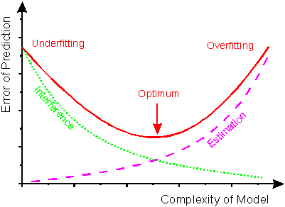
Specificity: predicted false / total false ROC curve = fpr (false predicted value) v.s. ppr (positive predicted value) For a given Y_true and Y_score, the ROC curve is plotted by changing the threshold of the mapping from Y_score to Y_predict, (remember that we are working on classification) And it begins with a high threshold and end up with a low threshold, so at first, almost everypoint is defined as zero. so ppr and fpr both are zero, so this is the reason why ROC curve start from zero. Similarly it ends up at 1,1. BiAS AND VARIANCE TRADE OFF Basic question in machine learning is // y = f(x) + random error given data xi, yi estimate a model fN(x) // Minimizing the expectation of difference between prediction and true observation, which is found to be Bias**2 + Variance of the model itself + irreducible error(chaotic nature that cannot be removed) Do a mind experiment: a simple model such as linear regression, given N points, try a linear regression. On one hand, linear model will be dependent on the training dataset you have in hands. So there is a variability in your linear model, this is called variance of the model itself. On the other hand, the distance between the regression line and training dataset, can be described as a L2 error. A nature instinct is the deviation of data away from the straight line. In total, they will be bias error. According to Wiki, can be thought as the error caused by the simplifying assumptions built into the method. E.g., when approximating a non-linear function f(x) using a learning method for linear models, there will be error in the estimates f(x) due to this assumption. How to measure bias error and variance error?
Be careful! Even if the principle behind the wheel is a relation that independent of the training data, even if it was extremely simple, the method you choose for determining the true model (ML), actually determines what kind of variance you should expect. COMMENTS ON R2
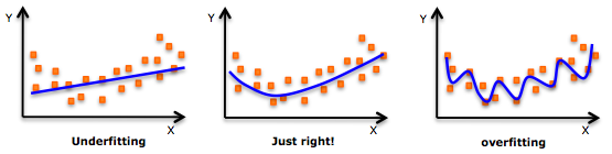
do we need to get more data? If you have 200 points, let say, it is good to try a cross validation with varying training sample size(also accomplished by sklearn learning curve), if predicted results has reached a extrema, then let's call it stop, because data is not that needed any more. so far the mdoel is good enough for current data. Adjusted R squared and r squared 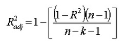 People realize that R squared in linear regression analysis can be misleading: -> adding more and more factors will ALWAYS increase the R squared, no matter it is useful or not. So how to choose a R squared that will guide us to add useful variable? ---> choose adjusted R squared. n is total number of samples, k is the number of factors in your regression model The mechanism is that adjusted R squared will only increase when you add the right variable, that causes R^2 to increase, then it overweights the increase of k, resulting a increased adjusted R squared. For more information, visit: http://www.statisticshowto.com/adjusted-r2/ uNDerfitting and overfitting
  Ridge regression + lasso regression 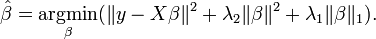 bai Both ridge and lasso are regularization of linear regression to reduce variance of the model. Ridge Ridge regression considers a penalty on L2 norm of coefficients in order to achieve reduced variance in models, based on the belief that smaller coefficient correlates closely to variance of model itself. Lasso Lasso model considers a L1 norm of penalty imposing on coefficient which based on the same argument for ridge. However, if there is a group of highly correlated variables, then the LASSO tends to select one variable from a group and ignore the others. The alpha is selected usually automatically to minimize the cross-validation error. Difference between Lasso and Ridge Lasso is able to achieve both of these goals by forcing the sum of the absolute value of the regression coefficients to be less than a fixed value, which forces certain coefficients to be set to zero, effectively choosing a simpler model that does not include those coefficients. This idea is similar to ridge regression, in which the sum of the squares of the coefficients is forced to be less than a fixed value, though in the case of Ridge regression, this only shrinks the size of the coefficients, it does not set any of them to zero. So in general, Lasso is an aggressive method, can select features, while Ridge is more conservative than Lasso, can only suppress overfitting. So if you are confident about the independence of your feature, use Ridge is safer than Lasso. Used as feature selection However! ONLY Lasso can be used as a tool of feature selection! If you try different alpha and plot the coef_ from fitted linear regressor, you will see as alpha increases, how does the coefficient vary and see if some feature can be eliminated at the first place. Elastic Net For a group of highly correlated data, lasso tends to eliminate all but one variable randomly. Elastic Net is the method of Ridge + Lasso, which is shown on the right. So Elastic Net can do feature selection, coefficient shrinkages. And the quadratic penalty term makes the loss function strictly convex, and it therefore has a unique minimum. So no random behaviour as Lasso. Stochastic Gradient Descent - SGD Regressor The class SGDRegressor implements a plain stochastic gradient descent learning routine which supports different loss functions and penalties to fit linear regression models. SGDRegressor is well suited for regression problems with a large number of training samples (> 10.000), for other problems we recommend Ridge, Lasso, or ElasticNet. So basically, it is still a linear model regressor but with fast speed. However, some tips has to be mentioned. Tip 1:
from sklearn.preprocessing import StandardScaler scaler = StandardScaler() scaler.fit(X_train) # Don't cheat - fit only on training data X_train = scaler.transform(X_train) X_test = scaler.transform(X_test) # apply same transformation to test data // For more information, please refer to http://scikit-learn.org/stable/modules/sgd.html PreprocessingTo generate features from raw data, in order to perform certain regression, preprocessing is used to generating those features. For example, for poly features, use the following command. pp_pf = preprocessing.PolynomialFeatures(degree=3) Also, if the input is more than one column, the result will contain interaction features. See the following in help documents. Generate polynomial and interaction features. Generate a new feature matrix consisting of all polynomial combinations of the features with degree less than or equal to the specified degree. For example, if an input sample is two dimensional and of the form [a, b], the degree-2 polynomial features are [1, a, b, a^2, ab, b^2]. classification LOGISTIC REGRESSION It sounds like it is a regression method but it is not. Actually regression is not that far away from classification. In some extent, they are almost the same. However, threshold is a interesting thing in classification, which also reflects how human classify things. This classification method, logistic regression, is actually mapping the whole Y results, into [0,1] using a exp function. Then linear fitting for a log function appear in the derivation process. Finally threshold considered as 0.5. So a classification result is coming into being. Some comments from Wiki I think is helpful:
Decision treeDecision tree learning uses a decision tree as a predictive model which maps observations about an item to conclusions about the item's target value. It is one of the predictive modelling approaches used in statistics, data mining and machine learning. Tree models where the target variable can take a finite set of values are called classification trees. In these tree structures, leaves represent class labels and branches represent conjunctions of features that lead to those class labels. Decision trees where the target variable can take continuous values (typically real numbers) are called regression trees. SVMMore formally, a support vector machine constructs a hyperplane or set of hyperplanes in a high- or infinite-dimensional space, which can be used for classification, regression, or other tasks. Intuitively, a good separation is achieved by the hyperplane that has the largest distance to the nearest training-data point of any class (so-called functional margin), since in general the larger the margin the lower the generalization error of the classifier.
Basic git command 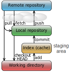 Fig 1. Fig 1. 1. git init: is used to create a local repo 2. git clone: if you have repo already in your github.. just use git clone and the address of your git. 3. git add : add the files to be tracked, add them into staging area (after I realize the structure of git, see Figure 1) 4. git remote add origin: it will connect the remote named as origin (this is used when you want to link a local repo to a repo in github) 5. git push -u origin master: will push the commits to origin and to the master branch (usually git push --all will push all the branches to remote) 6. git checkout -b branchname: it will create a new branch and GO THERE (git branch name will do the same thing but not checking out) 7. git rm: will delete the git tracking for a certain file AND delete the file Data dredging  I understand data dredging as, taking too much from the data than it actually contains. This idea also name as data fishing, data snooping, equation-fitting and p-hacking.. (I don't know the later two) The causes usually are drawing conclusions from non-representative data. PREDICTION V.S. INFERENCEThe difference is that prediction, is usually something in the future and can be validated easily. While inference, is something can perhaps never being verified. PYTHON PASS-BY-REFERENCE OR PASS BY VALUE? I found this problem when I tried to make a list with each element is a new list, where it contains a certain number of vectors.
The problem is solved by considering a 3D numpy array and work out by the way we do in MATLAB.. The cause is that Python automatically controls what to be pass-by-reference or by value. The thing we learnt for MATLAB is usually pass by value. However, list.append is a function could be pass-by-reference. import numpy as np from sklearn import linear_model, metrics, cross_validation import matplotlib.pyplot as plt %matplotlib inline np.random.seed(1) x = np.linspace(0, 6.14, 101) y = np.sin(x) + 0.3*np.random.randn(len(x)) N = 10 X = np.zeros((N,N,len(x))); trscore = np.zeros((N,1)) tescore = np.zeros((N,1)) trerr = np.zeros((N,1)) teerr = np.zeros((N,1)) aselect = np.add(range(N),1) for n in range(N): for i in range(n+1): if i == 0: X[n,i,:] = x else: X[n,i,:] = x**(i+1) for n_select in aselect: X_train, X_test, y_train, y_test = cross_validation.train_test_split(np.transpose(X[n_select-1])[:,0:n_select], y, test_size=0.33, random_state =48) lrg = linear_model.LinearRegression(n_jobs=-1) # print n_select,np.transpose(X[n_select-1])[:,0:n_select] lrg.fit(X_train,y_train) print 'when feature numer = ', n_select ,'abs(coef)_max = ', max(abs(lrg.coef_)) print 'when feature numer = ', n_select ,'abs(intercept)_max = ', max(abs(lrg.intercept_.ravel())) print '-------------------' tescore[n_select-1] = lrg.score(X_test,y_test) trscore[n_select-1] = lrg.score(X_train,y_train) trerr[n_select-1] = metrics.mean_squared_error(lrg.predict(X_test) ,y_test) teerr[n_select-1] = metrics.mean_squared_error(lrg.predict(X_train) ,y_train) fig = plt.figure(figsize=(16,4)) ax1 = fig.add_subplot(1,2,1) ax1.plot(aselect,tescore,c='blue',lw=3,label='test data') ax1.plot(aselect,trscore,c='red',lw=3,label='training data') ax1.legend(loc='best') ax1.set_xlabel('number of feature') ax1.set_ylabel('R2 score') ax2 = fig.add_subplot(1,2,2) ax2.plot(aselect, trerr, c='blue',lw=3,label='test data') ax2.plot(aselect, teerr, c='red',lw=3,label='training data') ax2.legend(loc='best') ax2.set_xlabel('number of feature') ax2.set_ylabel('MSE') |
AuthorShaowu Pan 
Archives
December 2017
Categories
All
|
 RSS Feed
